PCAone Tutorial (v0.7.0)
![]()
![]()
![]()


Introduction
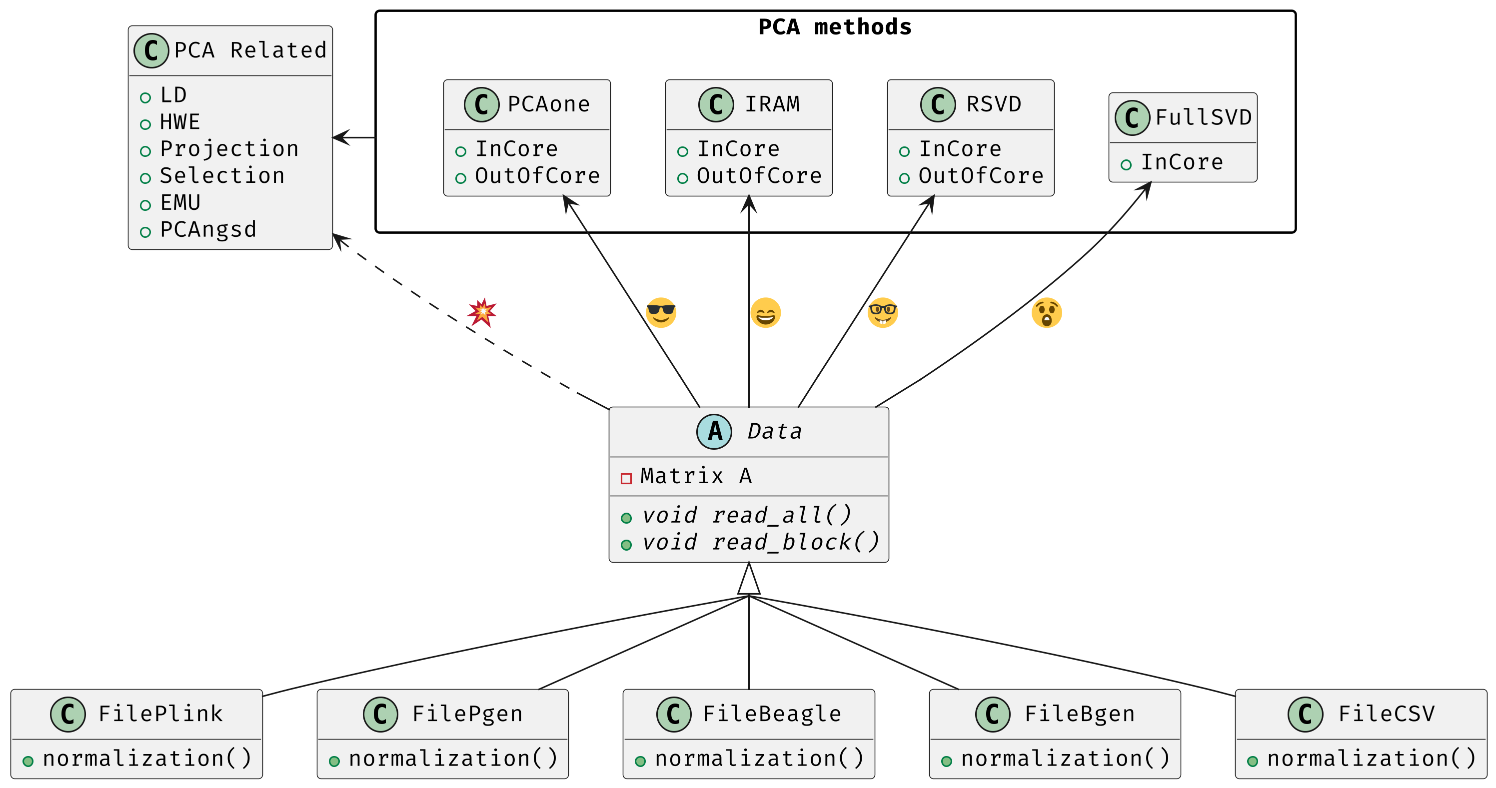
PCAone is a fast and memory efficient PCA tool implemented in C++ aiming at providing comprehensive features and algorithms for different scenarios. PCAone implements 3 fast PCA algorithms for finding the top eigenvectors of large datasets, which are Implicitly Restarted Arnoldi Method (IRAM, --svd 0), single pass Randomized SVD with power iteration scheme (sSVD, --svd 1, Algorithm1 in paper) and our proposed window based RSVD (winSVD, --svd 2, Algorithm2 in paper). All have both in-core and out-of-core implementation. Addtionally, Full SVD/Eigendecomposition (--svd 3) is supported via in-core mode only. Also, check out the R package here. PCAone supports multiple different input formats, such as PLINK BED, PLINK2 PGEN, BGEN, Beagle genetic data formats and a general comma separated CSV format for other data, such as scRNAs and bulk RNAs. For genetics data, PCAone also implements EMU and PCAngsd algorithm for data with missingness and uncertainty. The PDF manual can be downloaded here.
Features
See change log here.
- Has both Implicitly Restarted Arnoldi Method (IRAM) and Randomized SVD (RSVD) with out-of-core implementation.
- Implements our new fast window based Randomized SVD algorithm for tera-scale dataset.
- Quite fast with multi-threading support using high performance library MKL or OpenBLAS as backend.
- Supports the PLINK, BGEN, Beagle genetic data formats.
- Supports PLINK2 PGEN input via
--pgen, using dosages by default and hard calls with--hardcall. - Supports the comma separated CSV format with integer/float entries for single cell (or bulk) RNA-seq data compressed by zstd.
- Supports EMU algorithm for scenario with large proportion of missingness.
- Supports PCAngsd algorithm for low coverage sequencing scenario with genotype likelihood as input.
- Novel LD prunning and clumping method that accounts for population structure in the data.
- Projection support for data with missingness.
- Projection from BEAGLE genotype likelihoods onto a reference space via
--project 3. - HWE test taking population structure into account.
What's new in v0.7.0
- Added PLINK2
PGENinput support with--pgenfor PCA workflows. PGENreads dosages when available, and can be forced to use hard calls with--hardcall.- Added genotype-likelihood aware projection for
BEAGLEinput with--project 3. - Projection now matches overlapping markers against the reference
.mbimand corrects flipped alleles when needed. - Added genome-wide selection scans via
--selection 1(Galinsky/FastPCA) and--selection 2(pcadapt). - Bug fixes for projection with missing data
- Fast Eigendecomposition when
N<<Mwith-d 3
Cite the work
- If you use PCAone, please first cite our paper on genome reseach Fast and accurate out-of-core PCA framework for large scale biobank data.
- If using the EMU algorithm, please also cite Large-scale inference of population structure in presence of missingness using PCA.
- If using the PCAngsd algorithm, please also cite Inferring Population Structure and Admixture Proportions in Low-Depth NGS Data.
- If using the ancestry ajusted LD statistics for pruning and clumping, please also cite Measuring linkage disequilibrium and improvement of pruning and clumping in structured populations.
Quick start
pkg=https://github.com/Zilong-Li/PCAone/releases/latest/download/PCAone-avx2-Linux.zip
wget $pkg && unzip -o PCAone-avx2-Linux.zip
wget http://popgen.dk/zilong/datahub/pca/example.tar.gz
tar -xzf example.tar.gz && rm -f example.tar.gz
./PCAone -b example/plink
R -s -e 'd=read.table("pcaone.eigvecs2", h=F);
plot(d[,1:2+2], col=factor(d[,1]), xlab="PC1", ylab="PC2");
legend("topleft", legend=levels(factor(d[,1])), col=1:4, pch = 21, cex=1.2);'
You will find these files in current directory.
.
├── PCAone            # program
├── Rplots.pdf        # pca plot
├── example           # folder of example data
├── pcaone.eigvals    # eigenvalues
├── pcaone.eigvecs    # eigenvectors, the PCs you need to plot
├── pcaone.eigvecs2   # eigenvectors with header line
└── pcaone.log        # log file
\newpage
Installation
There are 3 ways to install PCAone.
Download compiled binary
There are compiled binaries provided for both Linux and Mac platform. Check the releases page to download one.
pkg=https://github.com/Zilong-Li/PCAone/releases/latest/download/PCAone-Linux.zip
wget $pkg || curl -LO $pkg
unzip -o PCAone-Linux.zip
Via Conda
PCAone is also available from bioconda.
conda config --add channels bioconda
conda install pcaone
PCAone --help
Build from source
PCAone has been tested on both Linux and MacOS system. To build PCAone from the source code, the following dependencies are required:
- GCC/Clang compiler with C++17 support
- GNU make
- zlib
On Linux, we recommend building the software from source with MKL as backend to maximize the performance.
With MKL or OpenBLAS as backend
Build PCAone dynamically with MKL can maximize the performance for large
dataset particularly, because the faster threading layer libiomp5 will be
linked at runtime. There are two options to obtain MKL library:
- download
MKLfrom the website
After having MKL installed, find the MKL root path and replace the path below with your own.
make -j4 MKLROOT=/opt/intel/oneapi/mkl/latest ONEAPI_COMPILER=/opt/intel/oneapi/compiler/latest
Alternatively, for advanced user, modify variables directly in Makefile and run make to use MKL or OpenBlas as backend.
- install
MKLby conda
conda install -c conda-forge -c anaconda -y mkl mkl-include intel-openmp
git clone https://github.com/Zilong-Li/PCAone.git
cd PCAone
# if mkl is installed by conda then use ${CONDA_PREFIX} as mklroot
make -j4 MKLROOT=${CONDA_PREFIX}
./PCAone -h
Without MKL or OpenBLAS dependency
If you don't want any optimized math library as backend, just run:
git clone https://github.com/Zilong-Li/PCAone.git
cd PCAone
make -j4
./PCAone -h
For MacOS users, check out the mac workflow.
brew install libomp
make -j4
\newpage
Documentation
Options
Run PCAone --groff > pcaone.1 && man ./pcaone.1 or PCAone --help to read the manual. Here are common options.
General options:
  -h, --help                     print all options including hidden advanced options
  -m, --memory arg (=0)          RAM usage in GB unit for out-of-core mode. default is in-core mode
  -n, --threads arg (=12)        the number of threads to be used
  -v, --verbose arg (=1)         verbosity level for logs. Options are
                                 0: silent, no messages on screen;
                                 1: concise messages to screen;
                                 2: more verbose information;
                                 3: enable debug information.

PCA algorithms:
  -d, --svd arg (=2)             SVD method to be applied. default 2 is recommended for big data. Options are
                                 0: the Implicitly Restarted Arnoldi Method (IRAM);
                                 1: the Yu's single-pass Randomized SVD with power iterations;
                                 2: the accurate window-based Randomized SVD method (PCAone);
                                 3: the full Singular Value Decomposition.
  -k, --pc arg (=10)             top k principal components (PCs) to be calculated
  -C, --scale arg (=-9)          do normalization or scaling for input file. Options are
                                 -9: standardize genetic data by sqrt(ploidy*f*(1-f));
                                  0: do nothing and proceed to SVD;
                                  1: do direct standardization, as the scale(x, center=TRUE, scale=TRUE) function in R;
                                  2: do first count per median log transformation (CPMED), then standardization;
                                  3: do first log1p transformation, then standardization;
                                  4: do first relative counts, then standardization.
  --maxp arg (=20)               maximum number of power iterations for RSVD algorithm.
  -S, --no-shuffle               do not shuffle columns of data for --svd 2 (if not locally correlated).
  --seed arg (=112)              seeds for reproducing results.
  --emu                          use EMU algorithm for genotype input with missingness.
  --pcangsd                      use PCAngsd algorithm for genotype likelihood input.

Input options:
  -b, --bfile arg                prefix of PLINK .bed/.bim/.fam files.
  -p, --pgen arg                 prefix of PLINK2 .pgen/.pvar/.psam files.
  -B, --binary arg               path of binary file.
  -c, --csv arg                  path of comma seperated CSV file compressed by zstd.
  -g, --bgen arg                 path of BGEN file compressed by gzip/zstd.
  -G, --beagle arg               path of BEAGLE file compressed by gzip.
  -F, --match-bim arg            the .mbim file to be matched, where the 7th column is allele frequency.
  -P, --USV arg                  prefix of PCAone .eigvecs/.eigvals/.loadings/.mbim.

Output options:
  -o, --out arg (=pcaone)        prefix of output files. default [pcaone].
  -V, --printv                   output the right eigenvectors with suffix .loadings.
  -D, --ld                       output a binary matrix for downstream LD related analysis.
  -R, --print-r2                 print LD R2 to *.ld.gz file for pairwise SNPs within a window controlled by --ld-bp.

Misc options:
  --maf arg (=0)                 exclude variants with MAF lower than this value
  --project arg (=0)             project the new samples onto the existing PCs. Options are
                                 0: disabled;
                                 1: by multiplying the loadings with mean imputation for missing genotypes;
                                 2: by solving the least squares system Vx=g. skip sites with missingness;
                                 3: by EM to account for genotype uncertainty (BEAGLE input).
  --inbreed arg (=0)             compute the inbreeding coefficient accounting for population structure. Options are
                                 0: disabled;
                                 1: compute per-site inbreeding coefficient and HWE test.
  --selection arg (=0)           compute selection statistics. Options are
                                 0: disabled;
                                 1: perform genome-wide selection scan using Galinsky et al method;
                                 2: perform genome-wide selection scan using pcadapt method.
  --ld-r2 arg (=0)               R2 cutoff for LD-based pruning (usually 0.2).
  --ld-bp arg (=1000000)         physical distance threshold in bases for LD window.
  --ld-stats arg (=0)            statistics to compute LD R2 for pairwise SNPs. Options are
                                 0: the ancestry adjusted, i.e. correlation between residuals;
                                 1: the standard, i.e. correlation between two alleles.
  --clump arg                    assoc-like file with target variants and pvalues for clumping.
  --clump-names arg (=CHR,BP,P)  column names in assoc-like file for locating chr, pos and pvalue.
  --clump-p1 arg (=0.0001)       significance threshold for index SNPs.
  --clump-p2 arg (=0.01)         secondary significance threshold for clumped SNPs.
  --clump-r2 arg (=0.5)          r2 cutoff for LD-based clumping.
  --clump-bp arg (=250000)       physical distance threshold in bases for clumping.
\newpage
Which SVD method to use
This depends on your datasets, particularlly the relationship between number
of samples (N) and the number of variants / features (M) and the top PCs
(k). Here is an overview and the recommendation.
| Method | Scenario | Accuracy | Speed |
|---|---|---|---|
| Full SVD (-d 3) | full variance explained | Exact | slow for big N and M |
| winSVD (-d 2) | M or N >> 500000 |
Very high | fast (only 7 iterations used) |
| IRAM (-d 0) | speed insensitive | Very high | denpends on N and # iterations |
| sSVD (-d 1) | accuracy insensitive | High | depends on # iterations |
Input formats
PCAone is designed to be extensible to accept many different formats.
Currently, PCAone can work with SNP major genetic formats to study
population structure. such as PLINK, BGEN and Beagle. Also, PCAone supports
a comma delimited CSV format compressed by zstd, which is useful for other
datasets requiring specific normalization such as single cell RNAs data. Since
v0.7.0, PCAone also supports PLINK2 PGEN
input via --pgen. If dosages are stored in the .pgen file, PCAone uses
them by default; add --hardcall to force hard-call genotypes instead. The
current BGEN support is limited, so for large production workflows we
recommend converting BGEN to PGEN when possible.
Output files
Eigen vectors
Eigen vectors are saved in file with suffix .eigvecs. Each row represents
a sample and each col represents a PC.
Eigen/Singular values
Eigenvalues and signularvalues are saved in file with suffix .eigvals and
.sigvals respectively. Each row represents the eigenvalue/singularvalue of
corresponding PC.
Features loadings
Features Loadings are saved in file with suffix .loadings. Each row
represents a feature and each column represents a corresponding PC. Use
--printv option to output it.
Variants infomation
A plink-like bim file named with .mbim is used to store the variants list
with extra information. Currently, the mbim file has 7 columns with the 7th
being the allele frequency. PCAone writes this file automatically whenever
it outputs .loadings via --printv, and for LD-related outputs that need
variant metadata downstream.
LD matrix
The matrix for calculating the ancestry-adjusted LD is saved in a file
with suffix .residuals, and its associated variants information is
stored in mbim file. For the binary file, the first
4-bytes stores the number of variants/SNPs, and the second 4-bytes stores
the number of samples in the matrix. Then, the rest of the file is a
sequence of M blocks of N x 4 bytes each, where M is the number of
variants and N is the number of samples. The first block corresponds to
the first marker in the .mbim file, etc.
LD R2
The LD R2 for pairwise SNPs within a window can be outputted to a file
with suffix ld.gz via --print-r2 option. This file uses the same long
format as the one plink used.
Performance and memory
PCAone has both in-core and out-of-core mode for 3 different partial SVD
algorithms, which are IRAM (--svd 0), sSVD (--svd 1) and winSVD (--svd 2).
Also, PCAone supports Full SVD (--svd 3) but with only in-core mode.
Therefore, there are 7 ways for doing PCA in PCAone. In default PCAone uses
in-core mode, which is the fastest way (NOTE: you can gain some speedup for
in-code computation by limiting the -n threads to half of the available
threads of your machine). However, in case the server runs out of memory,
you can trigger out-of-core mode by specifying the amount of memory using
-m/--memory option with a value greater than 0. Normally, use -m 1 is enough
for large dataset and PCAone will allocate more RAM when needed.
Run winSVD method (default) with in-core mode
./PCAone --bfile example/plink
Run winSVD method with out-of-core mode
./PCAone --bfile example/plink -m 2
Run sSVD method with out-of-core mode
./PCAone --bfile example/plink --svd 1 -m 2
Run IRAM method with out-of-core mode
./PCAone --bfile example/plink --svd 0 -m 2
Run Full SVD method with in-core mode
./PCAone --bfile example/plink --svd 3
Data Normalization
Note that data will be always first center for PCA. Additionally, there are
several different normalization method implemented with --scale option. One
should choose proper normalization method for specific type of data. In
default, PCAone will automatically apply the standard normalization for
genetic data.
Projection
Project new samples onto existing PCs is supported with --project option.
First, we run PCAone on a set of reference samples and output the loadings:
PCAone -b example/ref -k 10 --printv -o ref
Then, we need to read in the SNPs loadings from the ref set (--read-V) and
its scaling factors (--read-S) as well as the allele frequencies form the
.mbim file via --match-bim. You can use the --USV option instead to simplify
the usage since v0.4.8. For projection, PCAone matches overlapping markers
against the reference .mbim file and can correct flipped alleles when
needed, but you should still make sure both datasets are aligned to the same
genome build and alleles.
Below is a command using example PLINK data to project new target samples onto the reference coordinates.
PCAone -b example/new \
       --USV ref \      ## prefix to .eigvecs, .eigvals, .loadings, .mbim
       --project 2 \    ## check the manual on projection methods
       -o new
For BEAGLE genotype likelihood input, use --project 3 to perform
genotype-likelihood aware projection with an EM procedure:
PCAone -G example/target.beagle.gz \
       --USV ref \
       --project 3 \
       --scale 0 \
       -o target
Genome-wide selection scan
PCAone can test for differentiated variants after a good reference PCA has been computed with good sites after site-level QC, e.g. LD prunning.
First run PCA on the subset genotype matrix with good sites
PCAone -b example/subset -k 10 -o goodsites
Then reuse the saved USV outputs with --selection. Method 1 computes the
Galinsky/FastPCA statistic for each variant and PC, while method 2 computes
pcadapt-style z-scores, chi-square statistics, p-values, and a genomic
inflation factor.
PCAone -b example/fullset \
       --USV goodsites \
       --selection 1 \
       -o sel
PCAone -b example/fullset \
       --USV goodsites \
       --selection 2 \
       -o sel
The selection outputs are written per variant in the same marker order as the
plink .bim file.
HWE accounting for population structure
To test Hardy-Weinberg equilibrium in presence of population structure like pcangsd, we
need to work on the so-called individual allele frequencies matrix \(\Pi\),
which can be reconstructed via the output of PCAone, i.e the
.eigvecs,.sigvals,.loadings and .mbim files, generated by first running
PCAone -b example/plink -k 3 -V -o pcaone --pcangsd
## alternative for PLINK input with missingness
## PCAone -b example/plink -k 3 -V -o pcaone --emu
Then we apply --inbreed 1 option to obtain the P value of HWE and inbreeding
coefficient per-site. The per-site statistics is outputted to a file with suffix .hwe.
PCAone -b example/plink \
       --USV pcaone \
       --inbreed 1 \
       -o inbreed
Ancestry adjusted LD matrix
LD patterns vary across diverse ancestry and structured groups, and
conventional LD statistics, e.g. the implementation in plink --ld, failed to
model the LD in admixed populations. Thus, we can use the so-called
ancestry-adjusted LD statistics to account for population structure in
LD. See our paper for more details.
To calculate the ancestry-adjusted LD matrix, we first figure out the number
of principal components (-k/--pc) that capture population structure. In this
example, assuming that 3 PCs can accout for population structure, we enable
--ld option to calculate and output the ancestry adjusted LD matrix in a
file with suffix .residuals.
./PCAone -b example/plink -k 3 --ld -o adj
Report LD statistics
Currently, the LD R2 for pairwise SNPs within a window can be outputted via --print-r2 option.
./PCAone -B adj.residuals \
         --match-bim adj.mbim \
         --ld-bp 1000000 \
         --print-r2 \
         -o adj
We provide the calc_decay_bin.R script to parse the output file .ld.gz and calculate the average R2 for each
bin as well as plotting. We also provide the nextflow ld.nf for benchmarking the LD statistics.
Prunning based on ancestry adjusted LD
Given the LD binary file .residuals and its associated variant file
.mbim, we can do pruning based on user-defined thresholds and windows
./PCAone -B adj.residuals \
         --match-bim adj.mbim \
         --ld-r2 0.8 \
         --ld-bp 1000000 \
         -o adj
Clumping based on ancestry adjusted LD
Likewise, we can do clumping based on the Ancestry-Adjusted LD matrix and user-defined association results
./PCAone -B adj_ld.residuals \
         --match-bim adj.mbim \
         --clump example/plink.pheno0.assoc,example/plink.pheno1.assoc  \
         --clump-p1 0.05 \
         --clump-p2 0.01 \
         --clump-r2 0.1 \
         --clump-bp 10000000 \
         -o adj
More tutorials
Let's download the example data first if you haven't done so.
wget http://popgen.dk/zilong/datahub/pca/example.tar.gz
tar -xzf example.tar.gz && rm -f example.tar.gz
Genotype data (PLINK)
If you want to get the variance explained of each PC, we need to use --svd 3 to run Full SVD.
./PCAone --bfile example/plink -d 3
Then, we can make a PCA plot in R.
pcs <- read.table("pcaone.eigvecs2",h=F)
vals <- scan("pcaone.eigvals")
vals <- round(vals / sum(vals), 4)
xlab <- paste0("PC1: ", vals[1] * 100, "%")
ylab <- paste0("PC2: ", vals[2] * 100, "%")
plot(pcs[,1:2+2], col=factor(pcs[,1]), xlab = xlab, ylab = ylab, cex.lab = 1.5)
legend("topleft", legend=levels(factor(pcs[,1])), col=1:4, pch = 21, cex=1.2)
PLINK2 PGEN input
PCAone (version >= 0.7.0) can also read PLINK2 .pgen/.pvar/.psam input directly. By default it
uses dosages when they are present in the .pgen file.
./PCAone --pgen example/plink2_data -k 10 -m 2
If you want to ignore dosages and use hard-call genotypes instead, add
--hardcall.
./PCAone --pgen example/plink2_data -k 10 -m 2 --hardcall
BGEN input (limited support)
NB: BGEN support is very limited. Please convert BGEN to PGEN and use PGEN input!
Imputation tools usually generate the genotype probabilities or dosages in
BGEN format. To do PCA with the imputed genotype probabilities, we can
work on BGEN file with --bgen option instead.
./PCAone --bgen example/test.bgen -k 10 -m 2
Single cell RNA-seq data (CSV)
In this example, we run PCA for the scRNAs-seq data using CSV format with a
normalization method called count per median log transformation (CPMED).
Since the features (genes) tend to be not correlated locally, we use -S
option to disable permutation for winSVD.
./PCAone --csv example/BrainSpinalCord.csv.zst -k 10 -m 2 --scale 2 -S
Acknowledgements
PCAone uses Eigen for linear algebra operation. The IRAM method is based on yixuan/spectra. The bgen lib is ported from jeremymcrae/bgen. The EMU and PCAngsd algorithms are modified from @Jonas packages.
Contributing
PCAone is an open source project, and we welcome quality contributions. If you are interested in contributing and have experience with C++ (or LLM :D), feel free to reach out with ideas you would like to implement yourself.